
If you work a lot with Excel and manage large amounts of data, you sometimes need a little navigation aid. Such an aid can be a hyperlink that jumps to another worksheet in the same Excel file and navigates to a specific Excel cell and also highlights this cell. This can save a lot of time, especially with large files with a lot of data, because you don’t have to search and scroll for a long time.
What do we want to achieve?
As you can see in the following example GIF animation, a link and a link text are inserted in the first worksheet called “List“. If you click on this link, you automatically jump to the other worksheet “Performances” and to a specific cell there.
Of course, you can also use a shortcut to switch to another worksheet, but this does not offer the same convenience.
How it is implemented
Fortunately, Excel offers a suitable function for this, in addition to many other functions, such as backwards search. To implement the scenario shown above, use the hyperlink function in Excel with a specific notation. The Excel function can be seen in the following image.

Simply write in the relevant cell where the link should appear:
=HYPERLINK("[#]'NameTablesheet'!Cell"; "Linktext")
Ex:
=HYPERLINK("[#]'Performances'!A4"; "Performances 2")
The first parameter of the Excel function contains the link target. In this case, in the special notation with the hash in square brackets [#] followed by the name of the spreadsheet in single quotation marks followed by an exclamation mark and then the cell specification for the cell to be referenced.
The second parameter contains the link text as it should appear clickable in the cell.
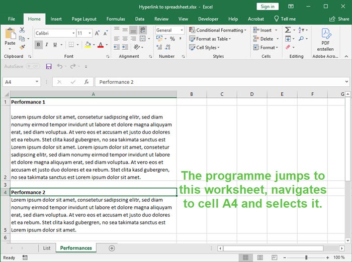
If you then click on the link, Excel automatically switches to the specified worksheet and the specified cell.
This is a very practical function which, if implemented correctly, can avoid a lot of searching and scrolling in large files.